C Chapter 6 Appendix

This appendix contains supplementary materials and analyses for the two experiments reported in Chapter 6.

C.1 Experiment 1

Below are hypotheses that were tested, but were not sufficiently relevant for Chapter 6 to be reported in the main text.

Hypothesis C.1 (Allocation similarity manipulation check for negative anecdote) For negative anecdotes, allocations for the anecdote only low similarity condition will be higher than those in the anecdote only high similarity condition.

Hypothesis C.2 (Relationship between allocation and perceived similarity for negative anecdote) In the negative valence condition, the correlation between allocation and similarity rating will be negative

Hypothesis C.3 (Relationship between allocation and specific-relevance for negative anecdote) In the negative valence condition, there will be no correlation between allocation and specific-relevance rating in the low similarity condition, but a negative correlation in the high similarity condition.

After the allocation task, participants were asked to rate the relevance of the anecdote to the target project. It was predicted that those that saw only an anecdote would be more influenced by the similarity of the anecdote than those that saw an anecdote as well as statistics. Therefore, the following hypotheses were tested:

Hypothesis C.4 The similarity effect on specific relevance will be greater in the anecdote only condition than in the anecdote + statistics condition.

Hypothesis C.5 The similarity effect on specific relevance will be greater in the statistics + anecdote condition than in the anecdote + enhanced statistics condition.

Further, participants were asked to rate the relevance of the anecdote to other projects in the same industry. It was predicted that those that saw only an anecdote would be more influenced by the similarity of the anecdote than those that saw an anecdote as well as statistics. Therefore, the following hypotheses are tested:

Hypothesis C.6 The similarity effect on general relevance will be greater in the anecdote only condition than in the anecdote + statistics condition.

Hypothesis C.7 The similarity effect on general relevance will be greater in the statistics + anecdote condition than in the anecdote + enhanced statistics condition.

C.1.1 Method

C.1.1.1 Participants

C.1.1.1.1 Power Analysis

The sample size for Experiment 1 was determined by conducting power analyses using the Superpower package (Lakens & Caldwell, 2019). The package uses experimental design, and predicted means and standard deviation, to conduct a priori power calculations. Data from Wainberg (2018), Jaramillo et al. (2019), and Hoeken and Hustinx (2009 Study 3) was used to determine realistic means and standard deviations for the evidence and similarity factors. According to the power functions, the resulting sample size is assumed to allow for an expected power of at least 80%.

Data from Wainberg (2018) were used to determine the predicted means for the anecdote conditions. Specifically, the values for the high similarity condition were taken from the anecdote & statistics, anecdote & enhanced statistics, and statistics only conditions for the corresponding anecdote conditions. This was done because in Wainberg (2018) the anecdote was always of a similar case. Wainberg (2018) did not use an anecdote only condition, but Wainberg et al. (2013) did and found no significant differences between the anecdote only condition and the anecdote & statistics condition. As such, the same mean value was used for both conditions.

It was hypothesised that there will only be an effect of similarity for the anecdote only and anecdote & statistics conditions. As such, the data from Hoeken and Hustinx (2009 Study 3) were used to determine the corresponding mean values for the low similarity condition. Specifically, each predicted mean was multiplied by the Cohen’s $d_z$ of the similarity effect in Hoeken and Hustinx (2009 Study 3).

To determine the predicted standard deviation, the data from Jaramillo et al. (2019) Experiment 2 and Hoeken and Hustinx (2009 Study 3) were re-analysed to determine the coefficient of variation (CV) of each condition. Each CV was then converted to a standard deviation value in the relevant scale by multiplying the mean of the CV values by the predicted means from above.

As shown in Figure C.1, the power analysis suggested that a minimum sample size of 294 (42 $\cdot$ 7) is required for the interaction effect with an expected power of at least 80%.

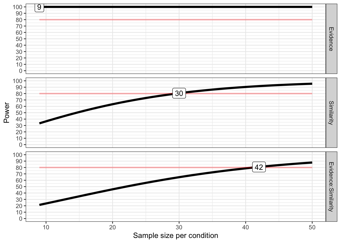
Figure C.1: Power curves for the similarity and anecdote effects.

C.1.1.2 Method

C.1.1.2.1 Instructions

Figure C.2 shows the general instructions all participants received, and Figures C.3, C.4, C.5, and C.6 show the condition-specific instructions.

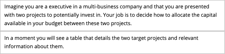
Figure C.2: Experiment 1 general instructions. The two boxes were split between two separate web-pages.

Figure C.3: Experiment 1 specific instructions for those in the anecdotes only condition.

Figure C.4: Experiment 1 specific instructions for those in the anecdote & statistics condition.

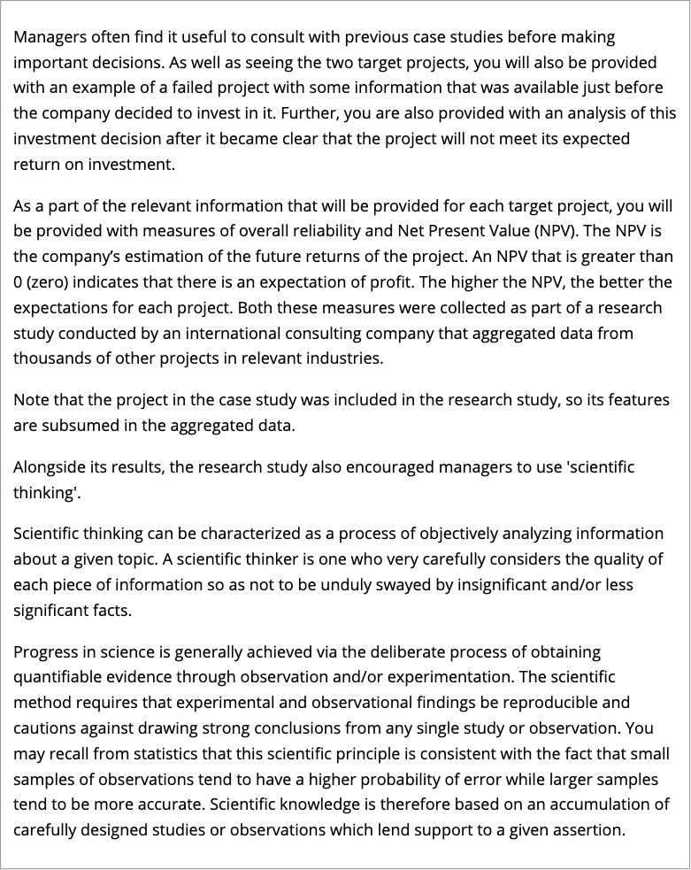
Figure C.5: Experiment 1 specific instructions for those in the anecdote & enhanced statistics condition.

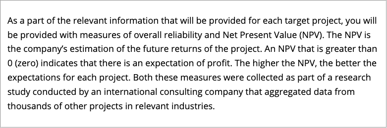
Figure C.6: Experiment 1 specific instructions for those in the statistics only condition.

C.1.1.2.2 Allocation Task

A horizontally integrated company is one which is made up of multiple businesses that operate in similar markets, and may have previously been competitors (Gaughan, 2012 a). A vertically integrated company, on the other hand, is one which is made up of multiple business than operate in the same market, but in different levels of the supply chain (Gaughan, 2012 b). A centralised organisational structure is one in which a company decisions tend to come from a specific business unit or leader, whereas a decentralised structure is one in which decisions can be made by separate units or people independently (Kenton, 2021).

C.1.1.2.3 Follow-up

Figure C.7 shows the follow-up questions.

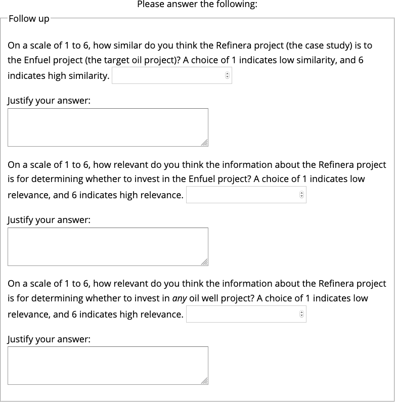
Figure C.7: Follow-up questions in Experiment 1.

C.1.2 Results

C.1.2.1 Allocation

A two-way ANOVA was conducted to investigate the interaction of similarity (low and high) and anecdote conditions (anecdote only, statistics & anecdote, anecdote & enhanced statistics). The main text reports the more relevant interaction that excludes the enhanced statistics condition. There was a main effect of anecdote type, $F(2, 238) = 14.47$, $p < .001$, $\hat{\eta}^2_p = .108$; and a main effect of similarity, $F(1, 238) = 38.91$, $p < .001$, $\hat{\eta}^2_p = .141$. However, the interaction was not significant, $F(2, 238) = 2.16$, $p = .118$, $\hat{\eta}^2_p = .018$. The difference between the anecdote only condition and the anecdote & enhanced statistics condition was not significant, $M = -9.24$, 95% CI $[-22.00,~3.51]$, $t(238) = -1.43$, $p = .155$.

C.1.2.2 Manipulation Check

Figure C.8 shows participants’ ratings of the similarity of the anecdote to the target project. As intended, participants in the high similarity condition rated the anecdote as more similar to the target project than those in the low similarity condition, $F(1, 238) = 27.01$, $p < .001$, $\hat{\eta}^2_p = .102$.

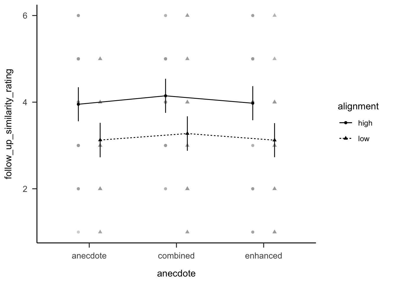
Figure C.8: Mean similarity rating of Project A (the target project) to the anecdote. Error bars represent 95% confidence intervals.

C.1.2.3 Follow-up

Figure C.9 shows participants’ ratings of the specific relevance question. There was no significant effect of evidence type $F(2, 238) = 0.96$, $p = .383$, $\hat{\eta}^2_p = .008$; or similarity, $F(1, 238) = 1.54$, $p = .216$, $\hat{\eta}^2_p = .006$. The interaction was also not significant, r results_anecdotes_1$relevance_specific$anecdote_alignment.

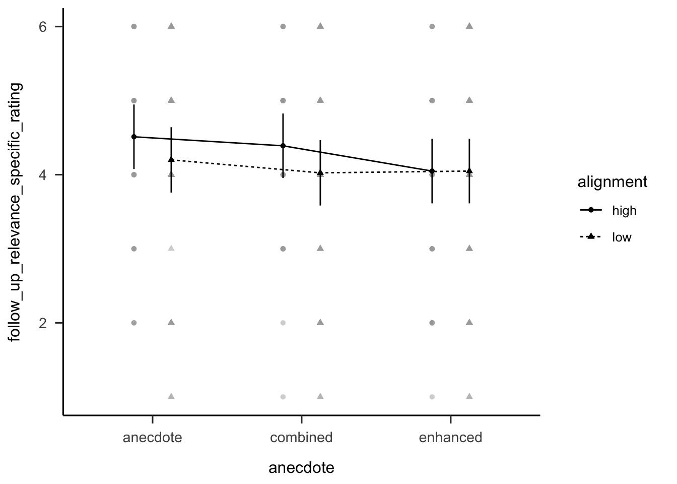
Mean rating of how relevant participants thought the anecdote was to Project A (the target project). Error bars represent 95% confidence intervals.

Figure C.9: Mean rating of how relevant participants thought the anecdote was to Project A (the target project). Error bars represent 95% confidence intervals.

Figure C.10 shows participants’ ratings of the general relevance question. There was no main effect of similarity, $F(1, 238) = 3.32$, $p = .070$, $\hat{\eta}^2_p = .014$, or interaction of similarity and evidence type, r results_anecdotes_1$relevance_general$anecdote_alignment. However, there was an unexpected main effect of evidence type, $F(2, 238) = 3.80$, $p = .024$, $\hat{\eta}^2_p = .031$. A contrast analysis with Bonferroni correction revealed that the anecdote only condition was rated significantly higher than the anecdote & statistics condition, $\Delta M = 0.58$, 95% CI $[0.06,~1.10]$, $t(238) = 2.71$, $p = .022$. However, the difference between the two anecdote & statistics conditions was not significant, $\Delta M = -0.39$, 95% CI $[-0.90,~0.13]$, $t(238) = -1.81$, $p = .212$.

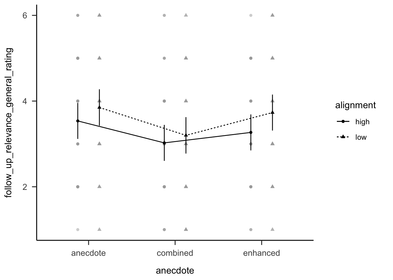
Mean rating of how relevant participants thought the anecdote was to other oil projects. Error bars represent 95% confidence intervals.

Figure C.10: Mean rating of how relevant participants thought the anecdote was to other oil projects. Error bars represent 95% confidence intervals.

Regression analyses were conducted to determine the relationship between allocations and the follow-up ratings of similarity and relevance. As shown in Figure C.11, similarity ratings were negatively correlated to allocations, $b = -3.53$, 95% CI $[-5.70, -1.37]$, $t(242) = -3.21$, $p = .002$. Finally, as shown in Figure C.12 similarity ratings were positively correlated to specific relevance ratings, $b = 0.30$, 95% CI $[0.17, 0.43]$, $t(242) = 4.59$, $p < .001$.

(ref:plot-anecdotes-1-lm-allocation-similarity) Mean allocation to the target project by similarity rating. The shading represents 95% confidence intervals.

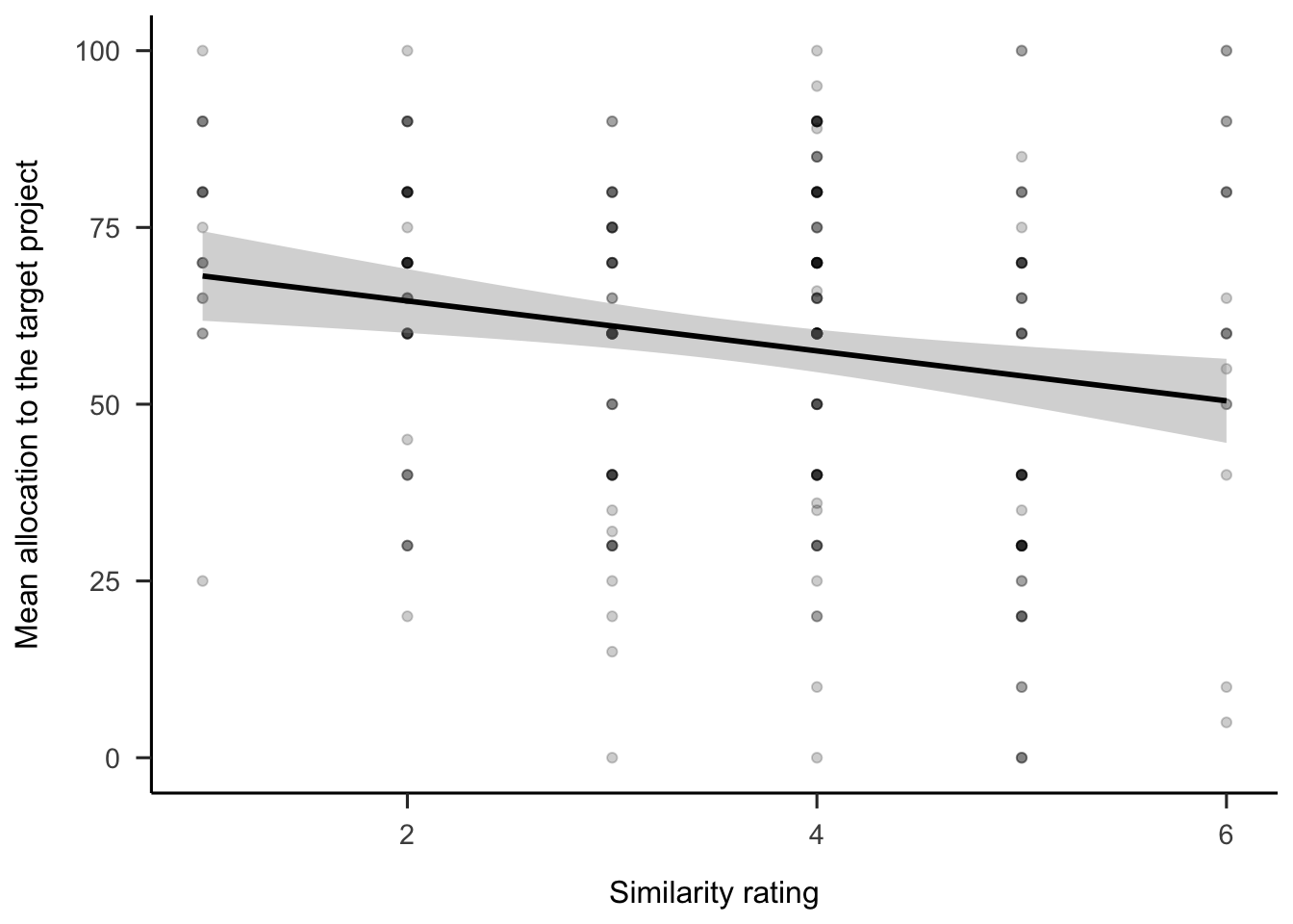
Figure C.11: (ref:plot-anecdotes-1-lm-allocation-similarity)

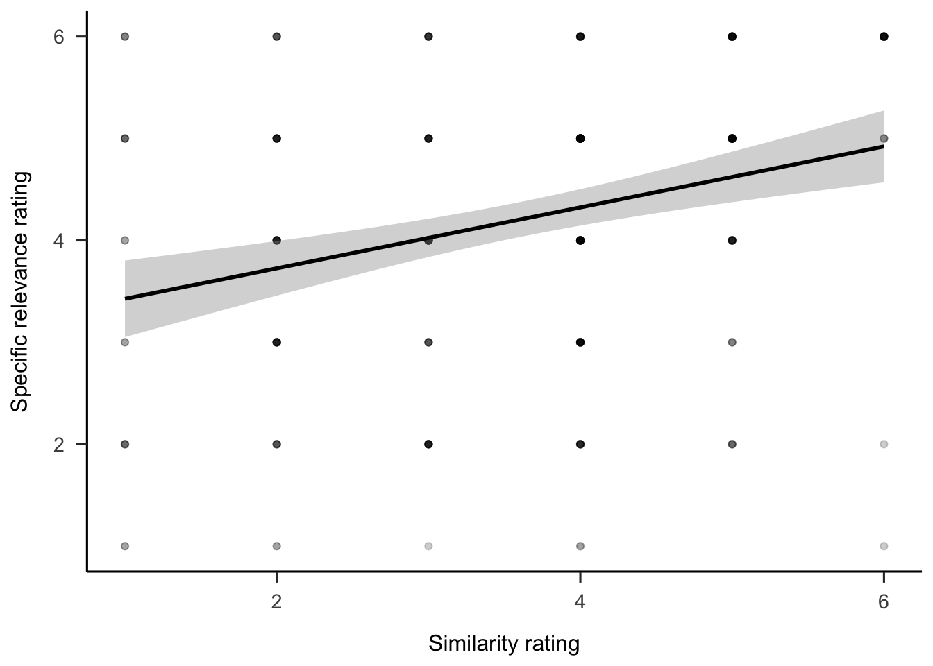
Rating of how relevant participants considered the anecdote to the target project, by similarity rating. The shading represents 95% confidence intervals.

Figure C.12: Rating of how relevant participants considered the anecdote to the target project, by similarity rating. The shading represents 95% confidence intervals.

Participants’ justifications for the ratings were not analysed, so are not reported.

C.2 Experiment 2

Figures C.13 and C.14 show the simulated data for the negative and positive valence conditions, respectively. These figures are different from the equivalent figures in the main text. Here, the same statistics only value was used for both valence conditions, whereas in the main text the relevant values for each condition were used. Further, the main text reports the difference score from the relevant statistics only values, whereas here the raw means are shown.

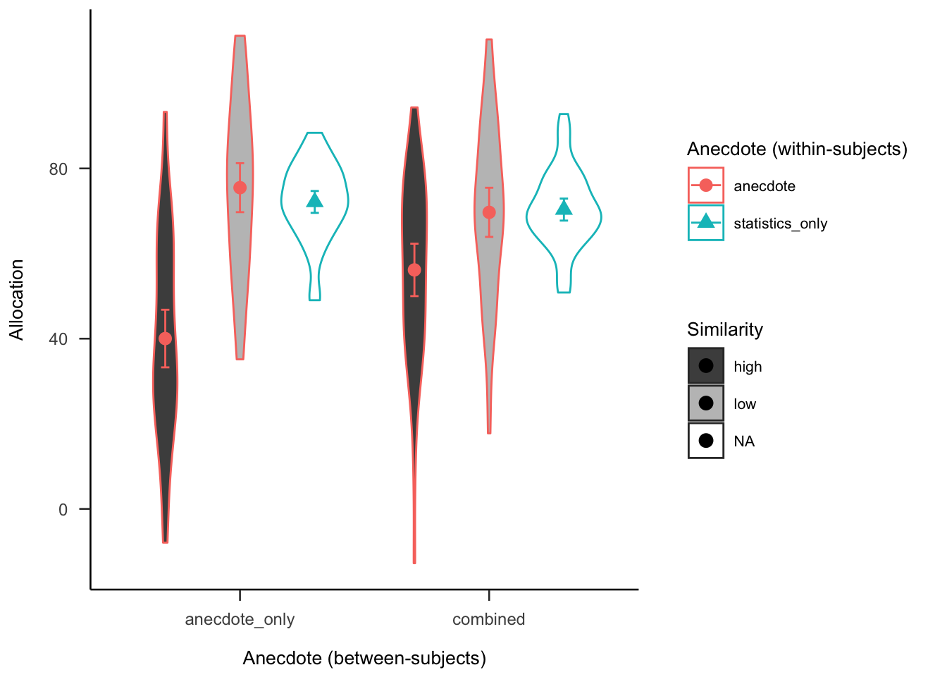
Figure C.13: Anecdotes Experiment 2 predicted data for the negative valence condition

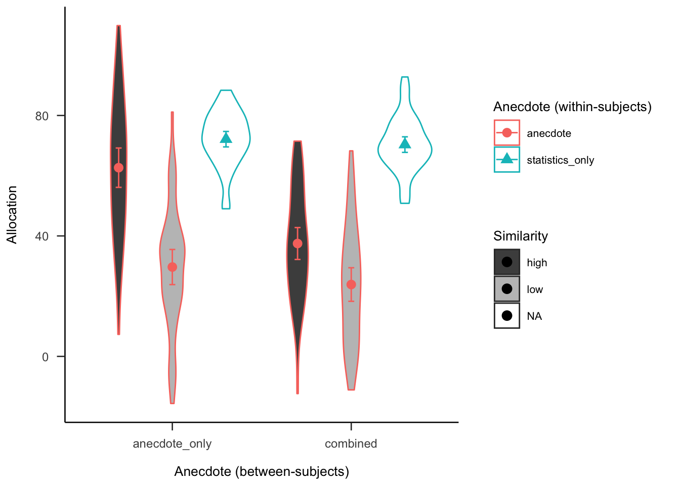
Figure C.14: Anecdotes Experiment 2 predicted data for the positive valence condition

Hypothesis C.8 (Allocation similarity manipulation check for positive anecdote) For positive anecdotes, allocations for the anecdote only high similarity condition will be higher than those in the anecdote only low similarity condition.

The rating effects found in Experiment 1 were expected to replicate in the Experiment 2 negative valence condition. The reverse effects were expected to be found in the positive valence condition.

Hypothesis C.9 (Relationship between allocation and perceived similarity for positive anecdote) In the positive valence condition, the correlation between allocation and similarity rating will be positive

Hypothesis C.10 (Relationship between allocation and specific-relevance for positive anecdote) In the positive valence condition, there will be no correlation between allocation and specific-relevance rating in the low similarity condition, but a positive correlation in the high similarity condition.

Hypothesis C.11 (Relationship between allocation and general-relevance for positive anecdote) There will be no significant correlations between allocation and general-relevance rating

C.2.1 Method

C.2.1.1 Participants

C.2.1.1.1 Power Analysis

A power analysis was conducted through simulation of the effects implied by the hypotheses in Experiment 2. Data were simulated with the same mean values as Experiment 1 for the effects that were previously significant (i.e., similarity, statistics, and interaction effects), and no effect for the differences that were non-significant (as shown in Figures C.13 and C.14). The null effect was analysed using the two one-sided tests (TOST) procedure, or equivalence testing (Lakens et al., 2018), and setting the smallest effect size of interest to the smallest difference that leads to a significant equivalence between the combined low similarity and statistics only conditions in Experiment 1. Figure C.15 shows the results of this analysis, which suggested a total sample size of 92 (46 $\times$ 2).

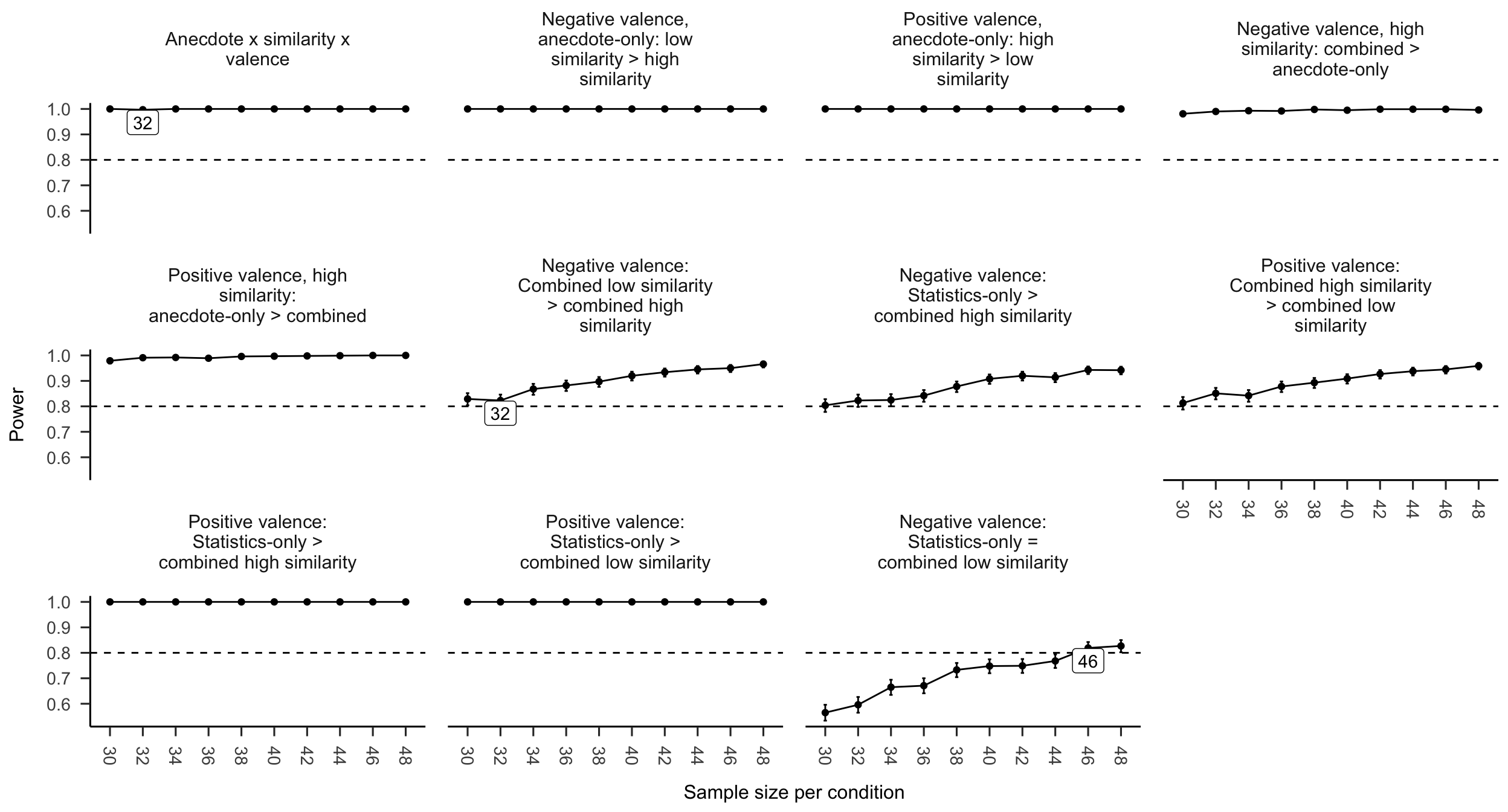
Figure C.15: Anecdotes Experiment 2 power curve. Labels indicate lowest sample size above 80% power.

C.2.1.2 Materials

C.2.1.2.1 Instructions

Figure C.16 shows the general instructions all participants received, and Figures C.17, C.18, and C.19 show the condition-specific instructions.

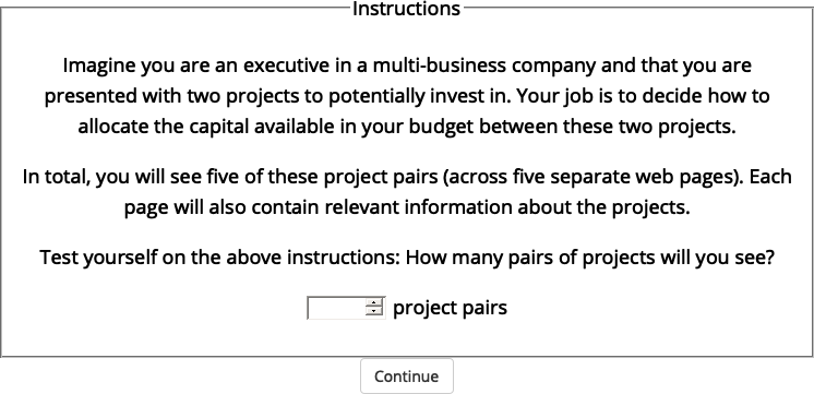
Figure C.16: General instructions for Experiment 2.

Figure C.17: Experiment 2 specific instructions for those in the anecdotes only condition.

Figure C.18: Experiment 2 specific instructions for those in the combined condition.

Figure C.19: Experiment 2 specific instructions for those in the statistics only condition.

C.2.1.2.2 Allocation Task

The following were counterbalanced: (a) project variation (five latin square variations), which is the association of each display content with each within-subject condition; and (b) anecdote variation (two variations), which is the association of each project display and being either the target or comparison project. Table column order and project display order were randomised.

C.2.1.2.3 Follow-up Questions

Figure C.20 shows an example of the follow-up questions.

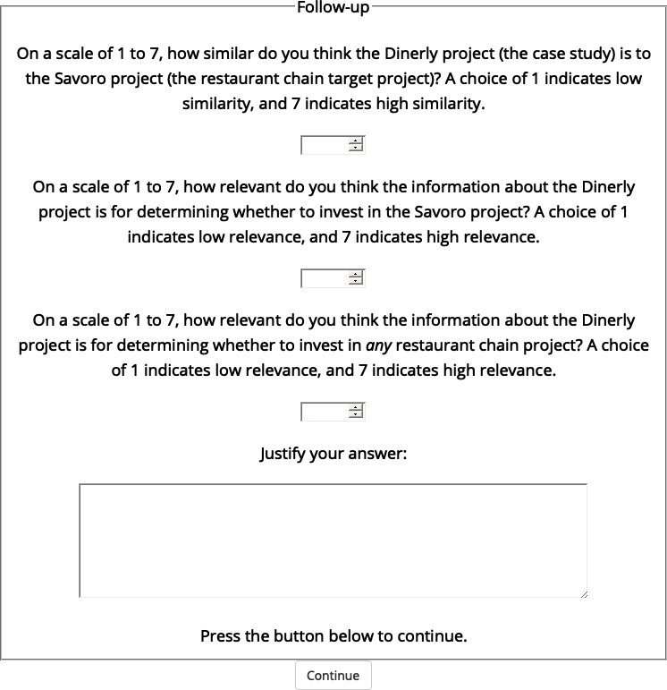
Figure C.20: An example of one of the follow-up question displays in Experiment 2.

C.2.1.2.4 Interstitial Display

Figure C.21 shows an example of one of the interstitial displays.

Figure C.21: An example of an interstitial display in Experiment 2.

C.2.2 Results

C.2.2.1 Allocation

C.2.2.1.1 Similarity Manipulation Check

The similarity manipulation worked as expected, with the negative anecdote only low similarity condition being allocated significantly more than those in the high similarity condition, $\Delta M = 26.98$, 95% CI $[18.12,~35.84]$, $t(186.55) = 6.01$, $p < .001$. For positive anecdotes, participants allocated more to the high similarity condition than those in the low similarity condition, $\Delta M = -22.62$, 95% CI $[-31.48,~-13.77]$, $t(186.55) = -5.04$, $p < .001$

C.2.2.2 Ratings

C.2.2.2.1 Similarity Manipulation Check

Evidence for the similarity manipulation working was also seen in the rating data. Participants rated anecdotes in the high similarity condition as more similar to the target than those in the low similarity condition, $F(1, 94) = 48.36$, $p < .001$, $\hat{\eta}^2_p = .340$.

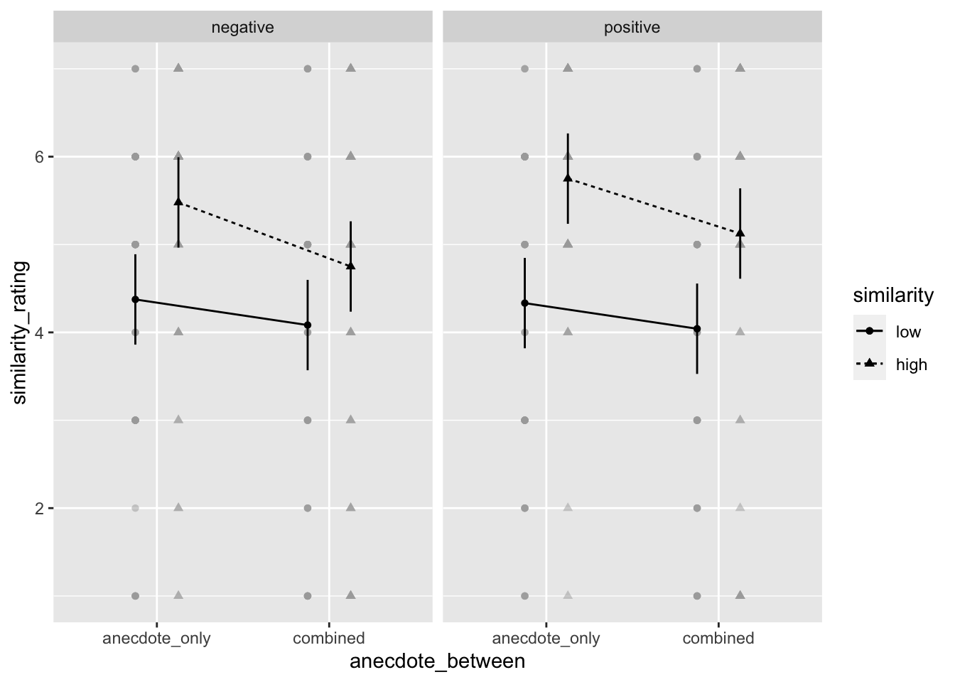
Figure C.22: Mean similarity rating of Project A (the target project) to the anecdote. Error bars represent 95% confidence intervals.

C.2.2.2.2 Allocation is Influenced by Perceived Similarity

As hypothesised, allocation was influenced by perceived similarity. That is, in the negative valence condition, there was a negative correlation between allocation and similarity rating, $\Delta M = 0.34$, 95% CI $[-3.72,~4.39]$, $t(376) = 0.16$, $p = .870$. However, in the positive valence condition, there was a positive correlation between allocation and similarity rating, $\Delta M = 2.86$, 95% CI $[-1.47,~7.18]$, $t(376) = 1.30$, $p = .195$.

C.2.2.2.3 The Relationship Between Allocation and Specific-Relevance Depends on Similarity

In the negative valence condition, there was no significant difference between the slopes of the high and low similarity conditions, $M = -2.02$, 95% CI $[-6.44,~2.41]$, $t(376) = -0.90$, $p = .371$. In the low similarity condition, allocation and specific-relevance rating were not correlated, $\Delta M = 1.01$, 95% CI $[-1.21,~3.22]$, $t(376) = 0.90$, $p = .371$, as in the low similarity condition, $\Delta M = -1.01$, 95% CI $[-3.22,~1.21]$, $t(376) = -0.90$, $p = .371$.

In the positive valence condition, there was no significant difference between the slopes of the high and low similarity conditions, $M = 4.25$, 95% CI $[-0.20,~8.70]$, $t(376) = 1.88$, $p = .061$. In the low similarity condition, allocation and specific-relevance rating were not correlated, $\Delta M = -2.12$, 95% CI $[-4.35,~0.10]$, $t(376) = -1.88$, $p = .061$, as in the low similarity condition, $\Delta M = 2.12$, 95% CI $[-0.10,~4.35]$, $t(376) = 1.88$, $p = .061$.

C.2.2.2.4 People do not Consider General-Relevance in Their Allocation

There were no significant correlations between allocation and general-relevance rating.

References

Gaughan, P. A. (Ed.). (2012a). Horizontal Integration and M&A. In Maximizing Corporate Value through Mergers and Acquisitions (pp. 117–157). John Wiley & Sons, Ltd. https://doi.org/10.1002/9781119204374.ch5

Gaughan, P. A. (Ed.). (2012b). Vertical Integration. In Maximizing Corporate Value through Mergers and Acquisitions (pp. 159–178). John Wiley & Sons, Ltd. https://doi.org/10.1002/9781119204374.ch6

Hoeken, H., & Hustinx, L. (2009). When is Statistical Evidence Superior to Anecdotal Evidence in Supporting Probability Claims? The Role of Argument Type. Human Communication Research, 35(4), 491–510. https://doi.org/10/fgtwjd

Jaramillo, S., Horne, Z., & Goldwater, M. (2019). The impact of anecdotal information on medical decision-making [Preprint]. PsyArXiv. https://doi.org/10.31234/osf.io/r5pmj

Kenton, W. (2021, March 1). How Organizational Structures Work. Investopedia. https://www.investopedia.com/terms/o/organizational-structure.asp

Lakens, D., & Caldwell, A. R. (2019). Simulation-Based Power-Analysis for Factorial ANOVA Designs [Preprint]. PsyArXiv. https://doi.org/10.31234/osf.io/baxsf

Lakens, D., Scheel, A. M., & Isager, P. M. (2018). Equivalence Testing for Psychological Research: A Tutorial. Advances in Methods and Practices in Psychological Science, 1(2), 259–269. https://doi.org/10/gdj7s9

Wainberg, J. S. (2018). Stories vs Statistics: The Impact of Anecdotal Data on Managerial Decision Making. In Advances in Accounting Behavioral Research (Vol. 21, pp. 127–141). Emerald Publishing Limited. https://doi.org/10.1108/S1475-148820180000021006

Wainberg, J. S., Kida, T., David Piercey, M., & Smith, J. F. (2013). The impact of anecdotal data in regulatory audit firm inspection reports. Accounting, Organizations and Society, 38(8), 621–636. https://doi.org/10/gjscqz

B Chapter @ref(alignment) Appendix

References