A Chapter 2 Appendix
This appendix contains supplementary materials and analyses for the two experiments reported in Chapter 2. In addition, it also report two experiments that were conducted to follow-up the findings in Experiments 1 and 2. Both follow-up experiments tested project choice as in the first two experiments, but Experiment 3 further investigated the effect of similarity, and Experiment 4 further investigated the effect of awareness.
All four experiments featured probability outcome distributions. These were
Poisson binomial distributions that were calculated using the R package
poibin, which uses calculations described in Hong (2013).
A.1 Experiment 1
A.1.1 Method
A.1.1.1 Materials
A.1.1.1.1 Instructions
Participants were shown the instructions in Figure A.1.

Figure A.1: Experiment 1 instructions.
A.1.1.1.2 Outcome Distribution Decision
Figure A.2 shows the outcome distribution display that participants saw in Experiment 1.
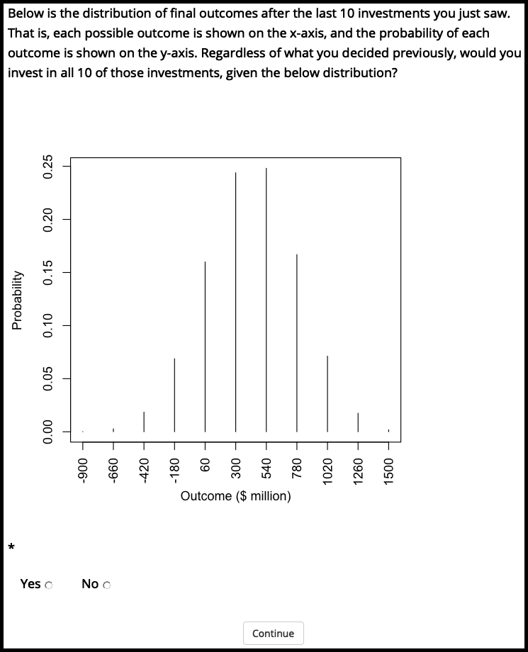
Figure A.2: The outcome distribution of the 10 gambles used in Experiment 1.
A.1.1.1.3 Follow-up Gambles
A.1.1.1.3.1 Negative EV Gambles
It was important to make sure that participants were generally making decisions that were in line with EV theory and that the sample was not abnormally risk tolerant. As such, participants saw two project decisions that had a negative EV. Out of the 396 negative EV gambles included (two per participant), all but four were rejected.
A.1.1.1.3.2 Samuelson (1963) Gambles
Participants saw the original Samuelson (1963) gamble, were asked whether they would accept 10 of that gamble, and whether they would accept those 10 given the associated outcome distribution. They then saw the same three questions, but using outcome magnitudes that were similar to the ones in the risky investment task. That is, $100 million instead of $100.
A.1.2 Results
A.1.2.1 Trial-by-Trial Analysis
Figure A.3 shows proportions of project acceptance across all conditions and trials.
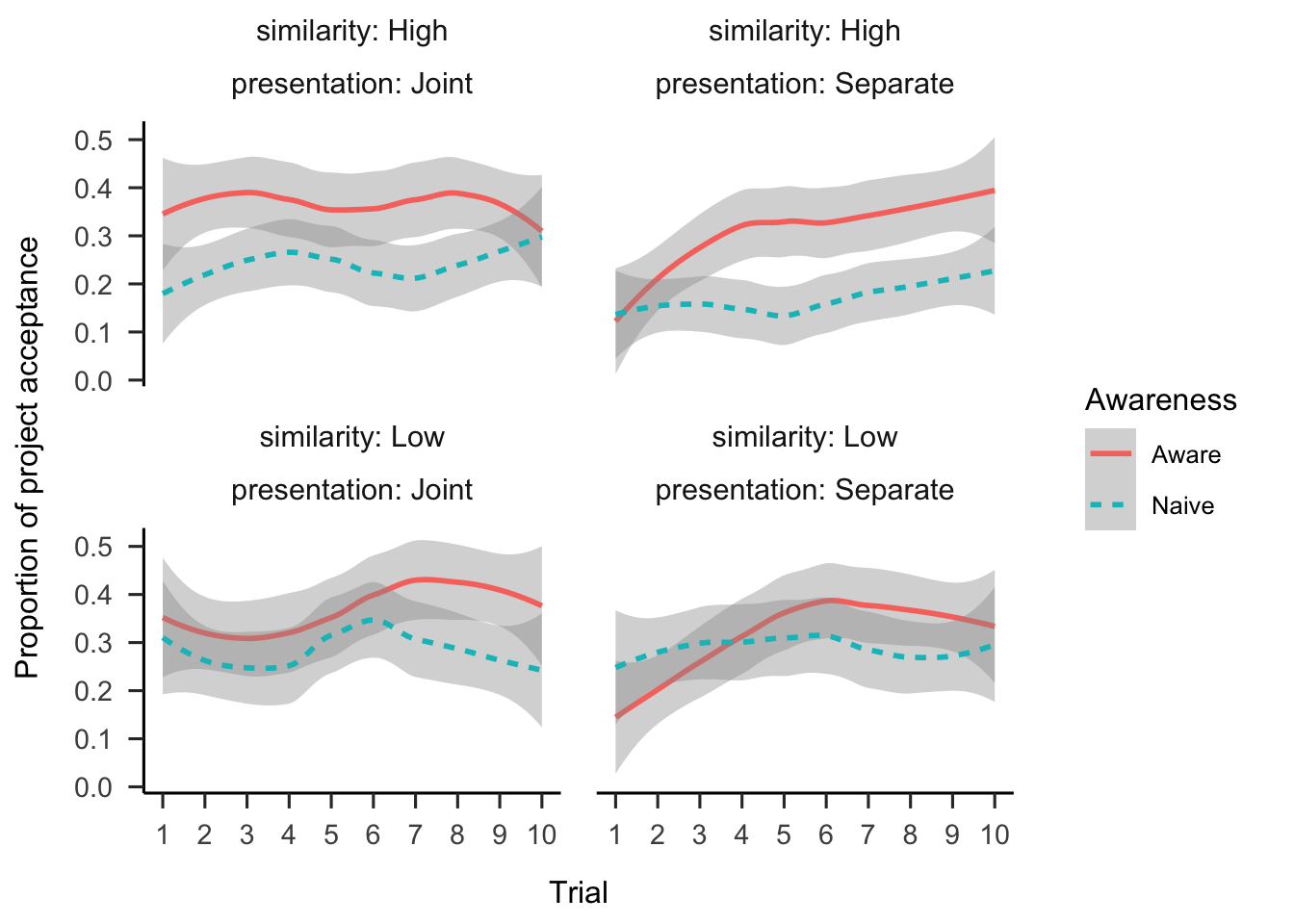
Figure A.3: Proportion of project acceptance by trial, similarity, awareness, and presentation conditions. LOESS is used for smoothing over trials, and the shading represents 95% confidence intervals.
A.1.2.2 Outcome Distribution
A paired-samples t-test was conducted to compare participants’ decision to invest in the 10 projects while seeing an aggregated distribution, and their decisions to invest in the projects individually, without the distribution. Participants invested in the 10 projects more when seeing the distribution both in the separate presentation phase, \(t(197) = 5.48\), \(p < .001\), \(d_z = 0.50\), 95% CI \([0.31, 0.68]\); and in the joint presentation phase, \(t(197) = 4.17\), \(p < .001\), \(d_z = 0.37\), 95% CI \([0.19, 0.56]\).
However, it was subsequently discovered that the code that generated this distribution mistakenly flipped the outcome values. This means that although it appeared from the distribution that the probability of loss was 0.09, the actual probability of loss of the underlying values given the correct distribution was 0.26. As such, even though Experiment 1 found an effect of distribution, it was unclear if the effect was driven by participants actually accurately assessing the riskiness of the individual gambles, and therefore showing a difference between the isolated and aggregated gambles in a normative way.
A.2 Experiment 2
A.2.1 Method
A.2.1.1 Participants
A.2.1.1.1 Power Analysis
The power analysis was conducted using the pwr package (Champely, 2020b), based
on the presentation effect size from Experiment 1, since it was the smallest
effect. The analysis suggested that a minimum sample size of
164 (41 \(\cdot\) 4) was required for
the presentation effect with an expected power of at least 80%.
A.2.1.2 Materials
A.2.1.2.1 Follow-up
Figure A.4 shows the project number question. The maximum value that they could enter was set to 20. Figures A.5 and A.6 ask participants whether they are willing to take all or none of the projects; and how many projects would they choose if they could pick randomly (maximum value was set to 20). Those in the distribution absent condition were asked the same questions, but without the distribution and its explanation.

Figure A.4: Experiment 2 project number question.
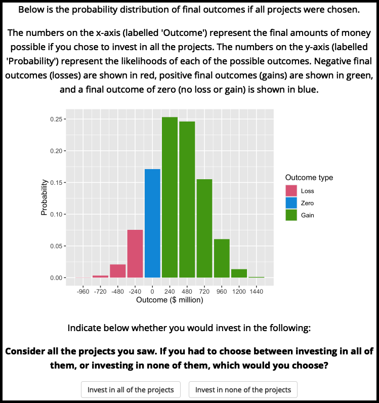
Figure A.5: Experiment 2 binary portfolio question.
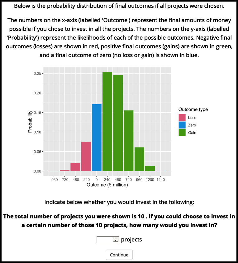
Figure A.6: Experiment 2 numerical portfolio question.
A.2.2 Results
A.2.2.1 Follow-up
A.2.2.1.1 Project Number
Participants were asked how many projects they thought they saw. Figure A.7 shows that overall people correctly estimated the number of projects, with more accuracy for those in the aware condition.
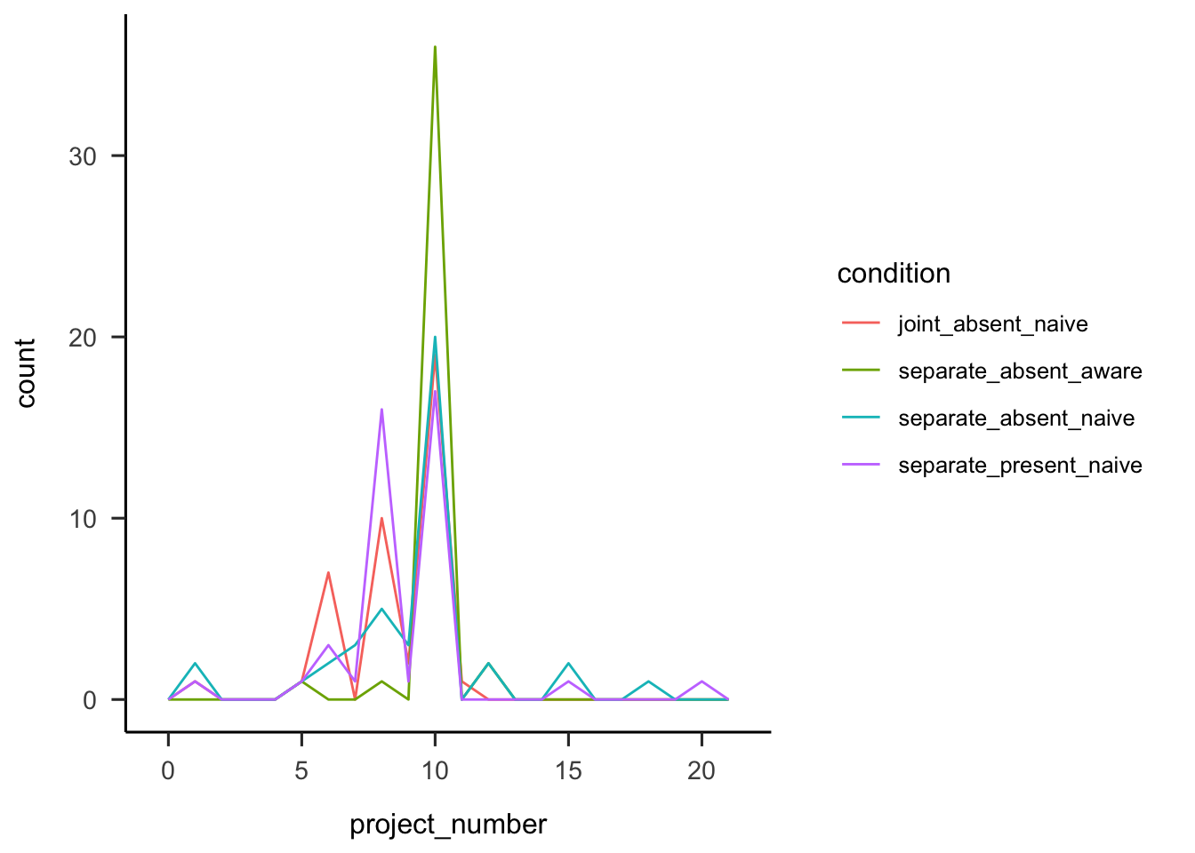
Figure A.7: Number of projects participants reported seeing, by condition.
A.2.2.1.2 Portfolio Choice - Binary
Participants were then asked if they would rather invest in all or none of the projects. As Figure A.8 shows, the difference between presentation conditions was not significant, \(\hat{\beta} = 0.15\), 95% CI \([-0.29, 0.60]\), \(z = 0.67\), \(p = .500\). The awareness effect was also not significant, \(\hat{\beta} = 0.28\), 95% CI \([-0.17, 0.72]\), \(z = 1.21\), \(p = .225\). However, those that that saw a distribution chose to invest in all 10 projects significantly more (71.43%) than those that did not see a distribution (36.59%), .
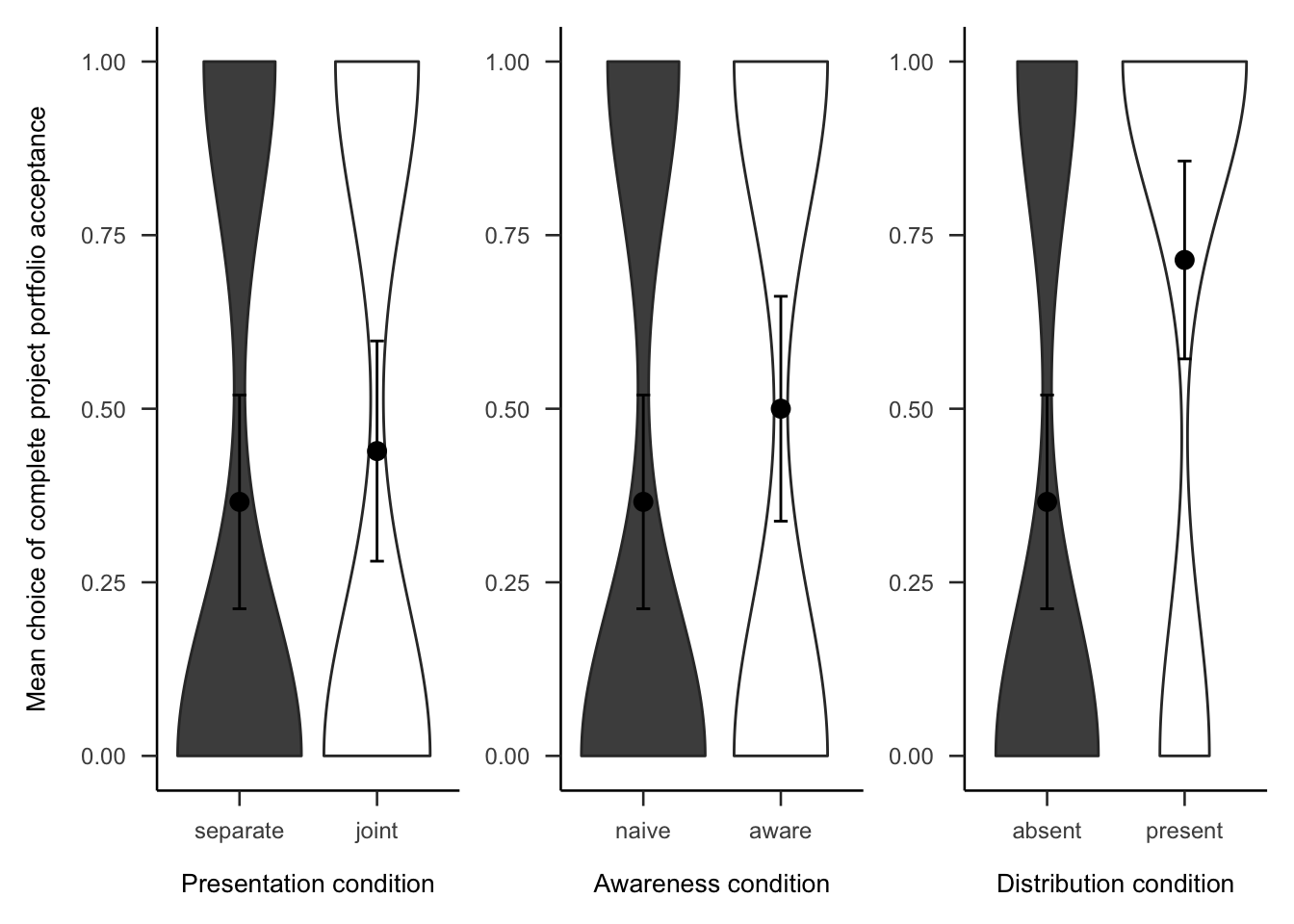
Figure A.8: Mean choice of investing in all 10 projects for the presentation, awareness, and distribution effects. Note, the condition on the left of each effect is the reference condition (separate presentation, naive awareness, distribution absent). As such, it is identical for the three effects.
A.2.2.1.3 Portfolio Choice - Number
Subsequently, participants were asked how many projects they would invest in out of the 10 that they saw. As Figure A.9 shows, the difference between presentation conditions was not significant, \(d_s\) = 0.08, 95% CI [-0.35, 0.52], \(t\)(80) = 0.38, \(p\) = .706. The awareness effect was also not significant, \(d_s\) = 0.09, 95% CI [-0.34, 0.53], \(t\)(79) = 0.42, \(p\) = .678. However, those that that saw a distribution chose to invest in significantly more projects than those that did not see a distribution, \(d_s\) = 0.60, 95% CI [0.15, 1.03], \(t\)(81) = 2.70, \(p\) = .009.
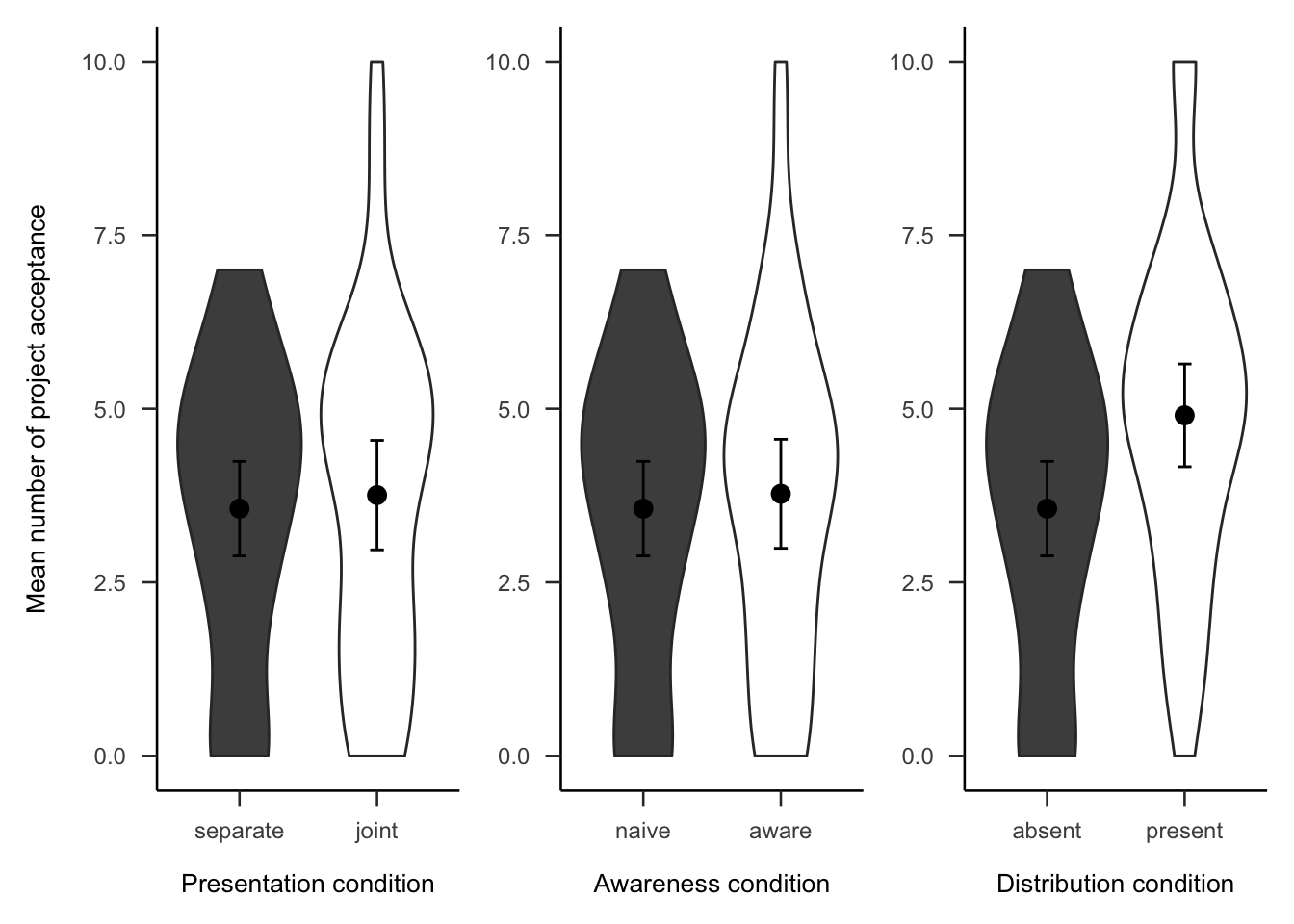
Figure A.9: Mean number of projects chosen in the follow-up for the presentation, awareness, and distribution effects. Note, the condition on the left of each effect is the reference condition (separate presentation, naive awareness, distribution absent). As such, it is identical for the three effects.
A.2.2.2 Gambles
Figures A.10 and A.11 show that the overall people seemed to prefer gambles with higher probabilities of gain, sometimes regardless of expected value or value of the gain.
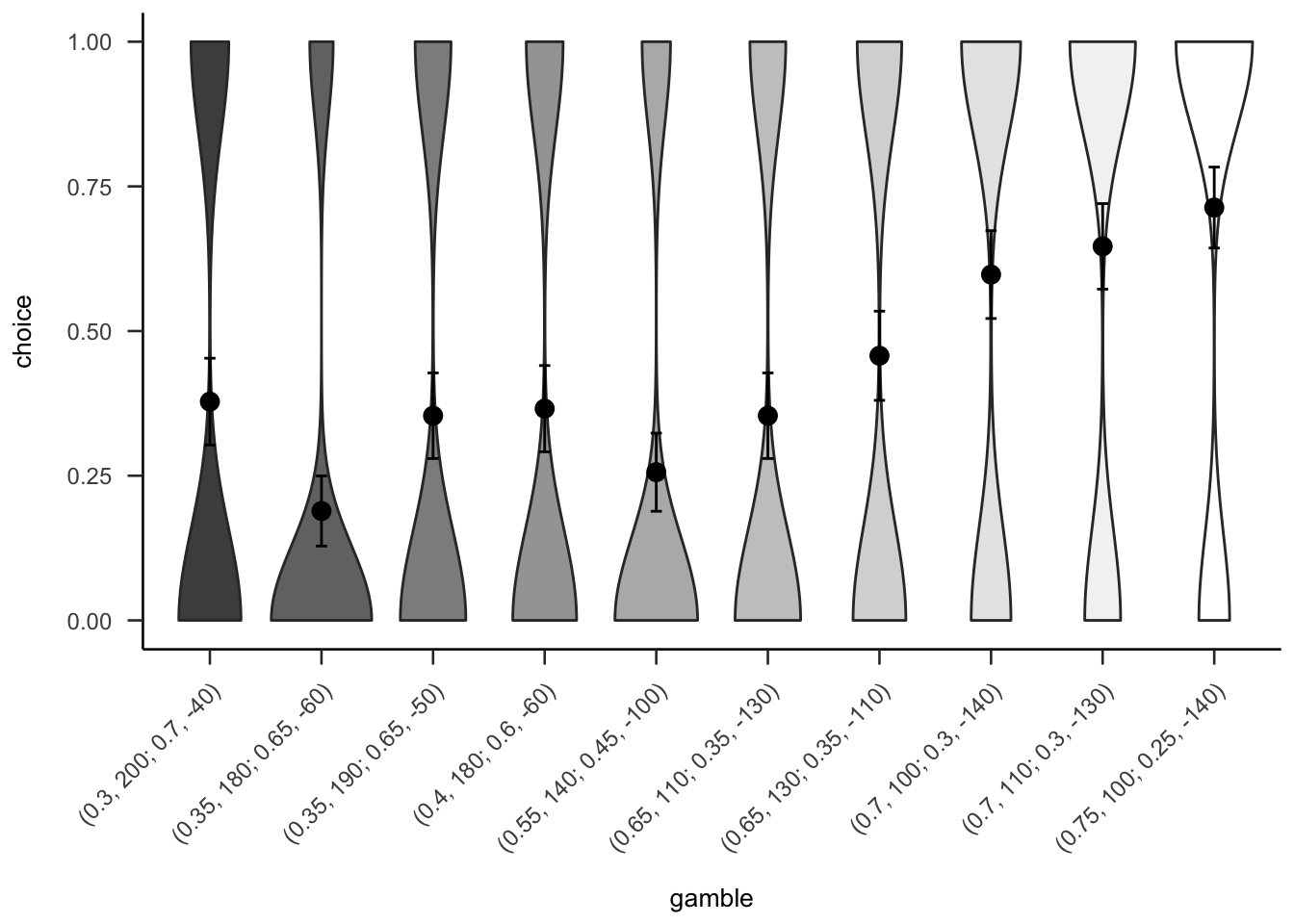
Figure A.10: Mean project acceptance for the 10 gambles. The format of the labels indicates: (gain probability, gain value; loss probability, loss value).
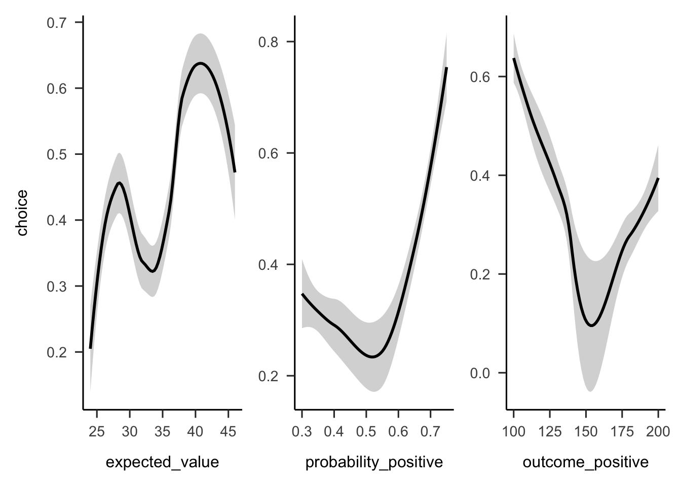
Figure A.11: Mean project acceptance for the gambles’ expected value, positive probability, and positive outcome.
A.3 Experiment 3
Experiment 3 investigated the effect of similarity on project choice. The previous experiments did not counterbalance the project domain when displaying the 10 projects to participants. Experiment 3 used 10 different potential business domains when constructing the project descriptions in order to reduce any potential effect that the specific domain may have on people’s choice. Therefore, Experiment 3 again tested Hypothesis 2.3.
A.3.1 Method
A.3.1.1 Participants
Two hundred and sixty-six participants (127 female) were recruited from the online recruitment platform Prolific. Participants were compensated at a rate of 5 an hour (Prolific is based in the UK). The average age was 39.56 years (SD = 8.77, min. = 25, max. = 71). Participants reported an average of 5.64 years (SD = 6.45, min. = 0, max. = 40) working in a business setting, and an average of 3.28 years (SD = 4.92, min. = 0, max. = 30) of business education. The mean completion time of the task was 9.23 min (SD = 7.2, min. = 1.41, max. = 65.46). Table A.1 shows the allocation of participants to the different conditions.
| Similarity | N |
|---|---|
| High | 133 |
| Low | 133 |
| Total | 266 |
A.3.1.2 Materials
A.3.1.2.1 Instructions
Participants were shown the same instructions as in Experiment 1 (see Section 2.2.1.2.1).
A.3.1.2.2 Risky Investment Task
Participants saw displays with the same gamble values as those in Experiment 2 (see Section 2.3.1.2.2), but with some changes in wording and sentence structure. The gamble information was the same, but extra prose was added to describe the projects. Further, the order of the sentences was randomised, so that the descriptions would not appear so similar. See Figure A.12 for an example.
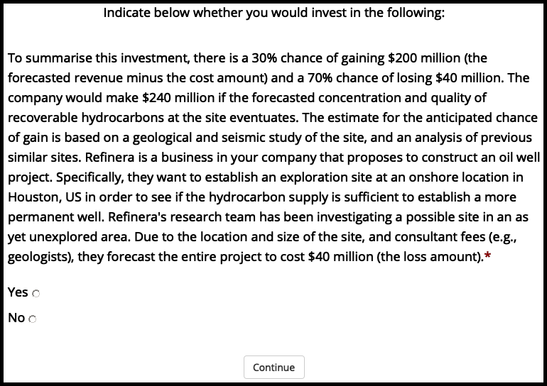
Figure A.12: An example of a project display in Experiment 3.
The similarity manipulation was as in Experiment 1. However, project domain was varied so that in the high similarity condition participants saw one of ten project domains.
A.3.1.2.3 Follow-up
The follow-up questions were similar to those in Experiment 2 (see Section 2.3.1.2.3), except in the portfolio number question participants were also shown the total number of projects that they saw (10). Further, another question was added, asking how many projects participants were expecting to see at the beginning of the experiment (see Figure A.13).

Figure A.13: Experiment 3 project expectation question.
A.3.2 Results
A.3.2.1 Project Investment
The project investment data were analysed as in Experiment 2 (see Section 2.3.2). Figures A.14 and A.15 show the choice and proportion data, respectively. The difference between similarity conditions was not significant, both in the logistic regression \(b = 0.00\), 95% CI \([-0.18, 0.17]\), \(z = -0.04\), \(p = .966\), and in the t-test, \(d_s\) = -0.21, 95% CI [-0.45, 0.03], \(t\)(264) = -1.69, \(p\) = .093.
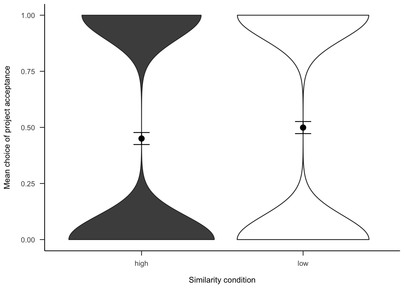
Figure A.14: Mean project acceptance for the similarity effect.
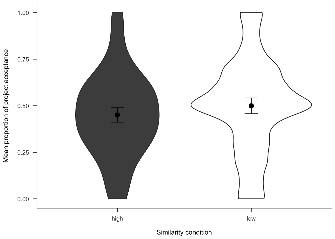
Figure A.15: Mean proportion of project acceptance for the similarity effect.
Further, Figure A.16 shows the choice data as a function of the order of the project in the sequence. As Table A.2 shows, there were no main effects or interactions.
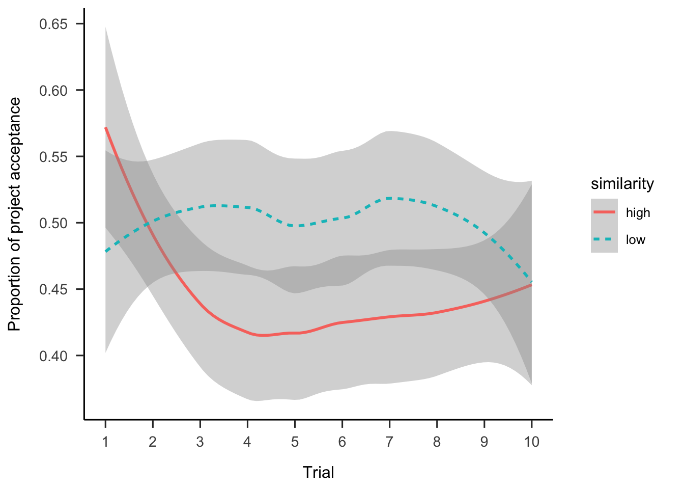
Figure A.16: Mean project acceptance by similarity and trial.
| Term | \(\hat{\beta}\) | 95% CI | \(z\) | \(p\) |
|---|---|---|---|---|
| Intercept | 0.01 | [-0.20, 0.22] | 0.07 | .944 |
| Similarity1 | -0.02 | [-0.23, 0.18] | -0.22 | .826 |
| Project order | -0.02 | [-0.05, 0.01] | -1.52 | .127 |
| Similarity1 \(\times\) Project order | -0.02 | [-0.05, 0.01] | -1.07 | .284 |
A.3.2.2 Follow-up
A.3.2.2.1 Project Expectation
Participants were asked how many projects they expected to see. As Figure A.17 shows, the difference between similarity conditions was not significant, \(d_s\) = -0.23, 95% CI [-0.47, 0.01], \(t\)(264) = -1.85, \(p\) = .065.
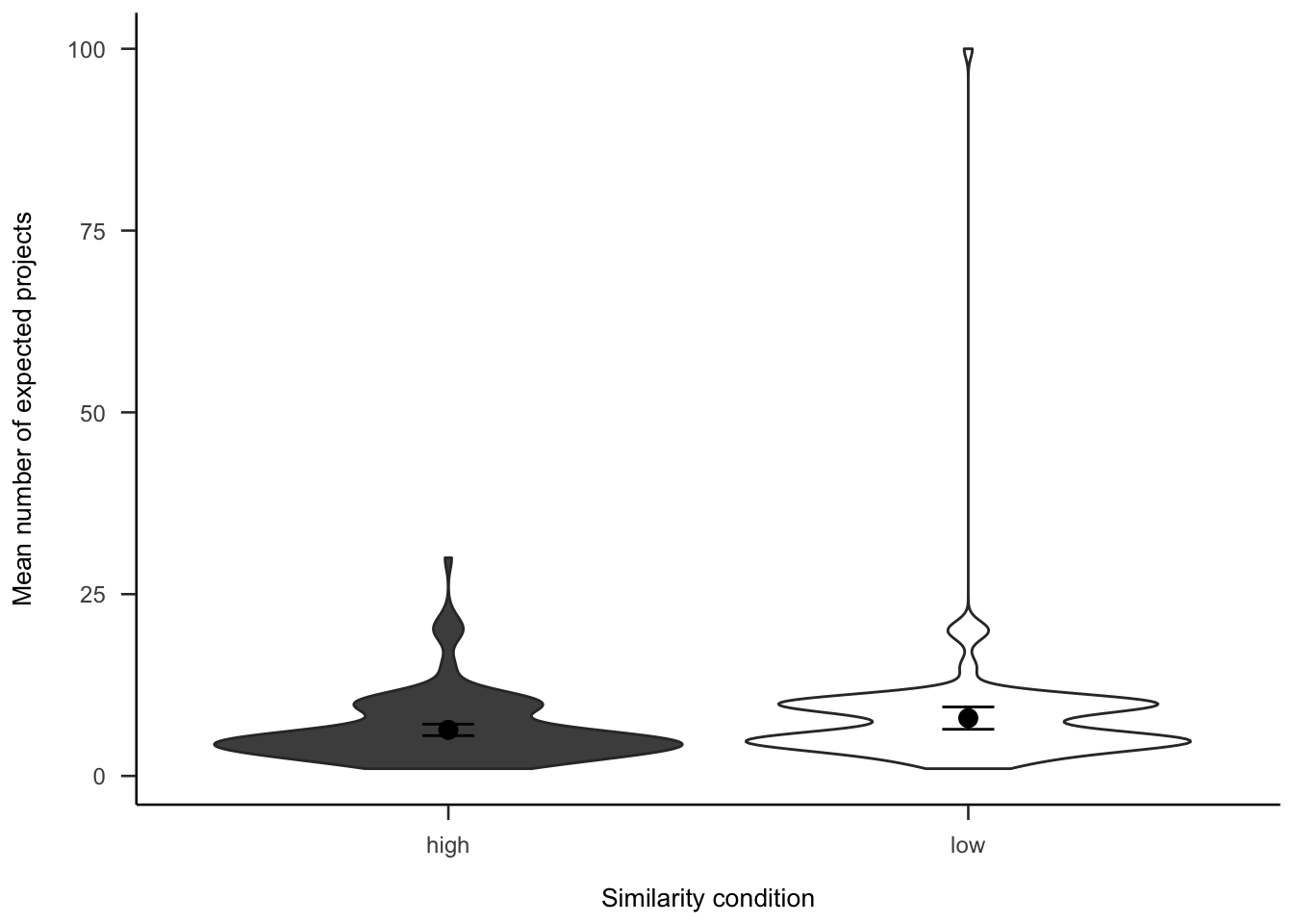
Figure A.17: Number of projects participants expected to see, by similarity.
A.3.2.2.2 Project Number
Participants were asked how many projects they thought they saw. Figure A.18 shows that overall people correctly estimate the number of projects.
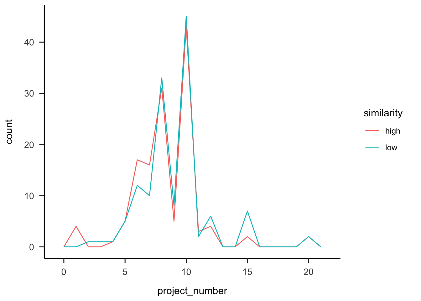
Figure A.18: Number of projects participants reported seeing, by similarity.
A.3.2.2.3 Portfolio Choice - Binary
Participants were then asked if they would rather invest in all or none of the projects. As Figure A.19 shows, those in the low similarity condition were significantly more likely to want to invest in all of the projects, \(b = -0.26\), 95% CI \([-0.51, -0.02]\), \(z = -2.10\), \(p = .036\).
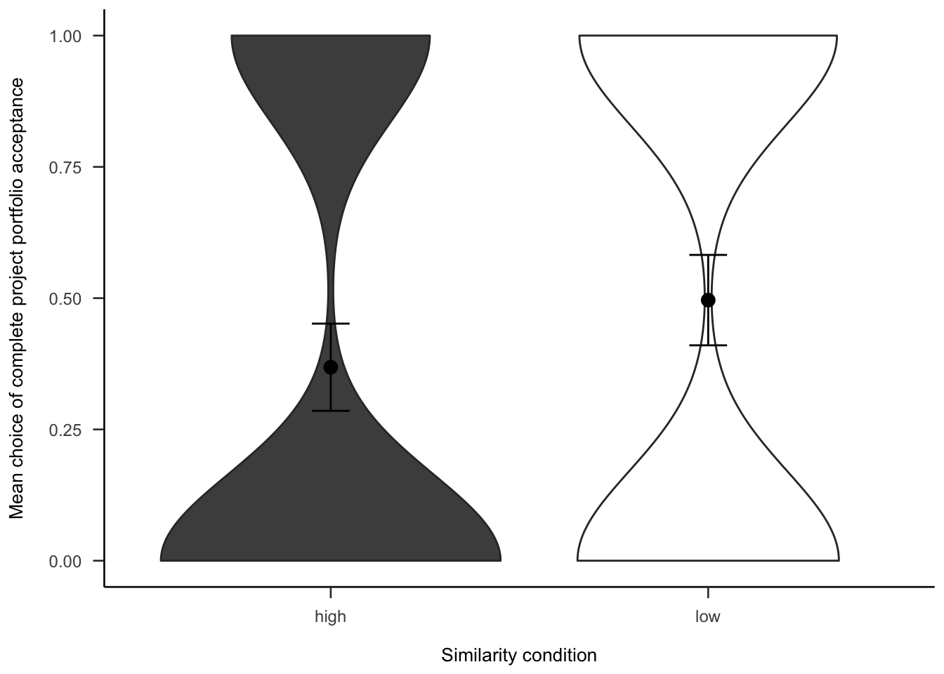
Figure A.19: Mean choice of investing in all 10 projects for the similarity effect.
A.3.2.2.4 Portfolio Choice - Number
Subsequently, participants were asked how many projects they would invest in out of the 10 that they saw. As Figure A.20 shows, the difference between similarity conditions was not significant, \(d_s\) = -0.14, 95% CI [-0.38, 0.10], \(t\)(264) = -1.12, \(p\) = .264.
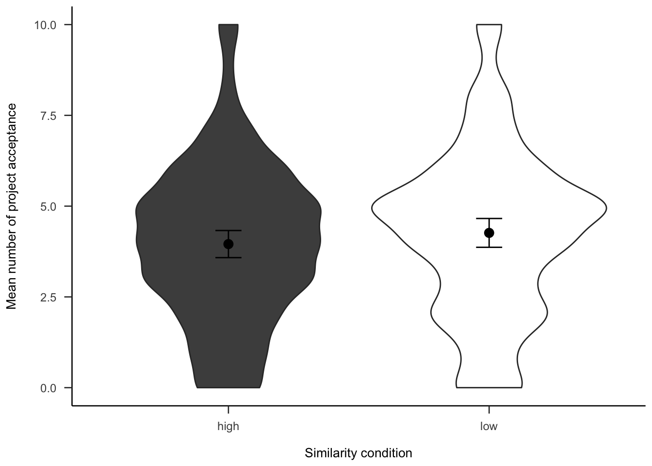
Figure A.20: Mean number of projects chosen in the follow-up for the similarity effect.
A.3.2.3 Gambles
Figures A.21 and A.22 show the overall people seemed to prefer gambles with higher probabilities of gain, sometimes regardless of expected value or value of the gain.
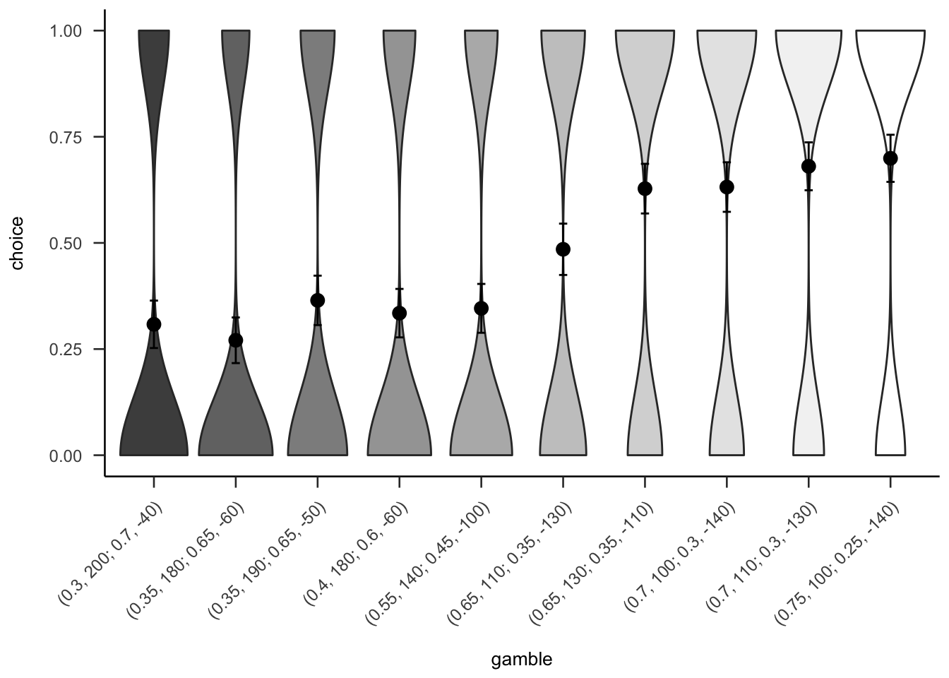
Figure A.21: Mean project acceptance for the 10 gambles. The format of the labels indicate: (gain probability, gain value; loss probability, loss value).
(ref:plot-aggregation-3-gamble-values) Mean project acceptance for the gambles’ expected value, positive probability, and positive outcome.
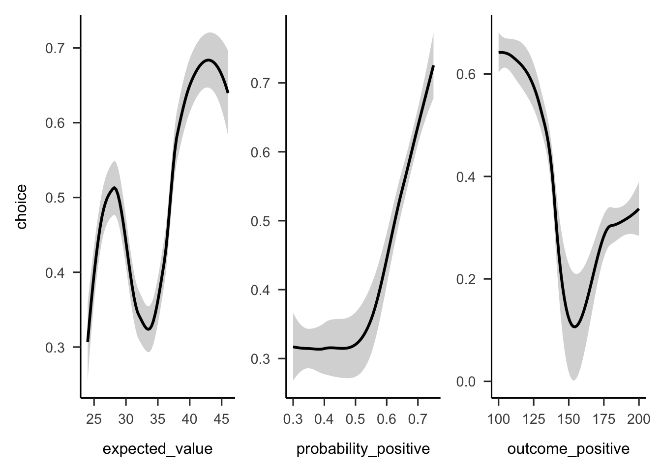
Figure A.22: (ref:plot-aggregation-3-gamble-values)
A.3.3 Discussion
Experiment 3 found some evidence for the effect of similarity on project choice, but it was in the opposite direction to the one hypothesised. Specifically, the results showed that when considering projects individually, participants’ risk aversion did not differ between similarity conditions, but when offered a portfolio of the projects, those that saw the dissimilar projects were more likely to invest.
These results provide evidence for the naive diversification account expressed above (see Section 2.2.3.3). Specifically, participants may really be naively diversifying, but only when they are explicitly given an opportunity to do so. This is similar to the multi-play effects because the question itself provides a sort of choice bracketing. That is, the gambles are grouped together as a portfolio by the question. Together, this suggests that people are not naively aggregating when viewing gambles in isolation, but when the choices are bracketed explicitly, then the choice seems to be driven by a naive diversification.
A.4 Experiment 4
Experiment 4 investigated the effect of awareness on project choice. Experiment 1 found an effect of awareness in the trial-by-trial data that was not replicated in Experiment 2. Above, this effect was explained through the law of small numbers: people may have been anticipating less risky gambles towards the end of the set. As such, the effect could be seen with more trials. Experiment 4 attempted to replicate the effect from Experiment 1 with 20 projects. The naive condition attempted to encourage participants to focus on projects one at a time and did not reveal the total number of projects. The aware condition attempted to encourage participants to think of all 20 projects. This was done by revealing the total number of projects in the beginning of the task and by identifying at each project display its order in the sequence. Experiment 4 again tested Hypothesis 2.4.
A.4.1 Method
A.4.1.1 Participants
Two hundred and sixty-six participants (110 female) were recruited from the online recruitment platform Prolific. Participants were compensated at a rate of 5 an hour (Prolific is based in the UK). The average age was 40.62 years (SD = 9.59, min. = 25, max. = 74). Participants reported an average of 7.45 years (SD = 7.8, min. = 0, max. = 47) working in a business setting, and an average of 5.52 years (SD = 7.27, min. = 0, max. = 48) of business education. The mean completion time of the task was 12.66 min (SD = 8.26, min. = 1.48, max. = 53.47). Table A.3 shows the allocation of participants to the different conditions.
| Awareness | N |
|---|---|
| Aware | 133 |
| Naive | 133 |
| Total | 266 |
A.4.1.2 Materials
A.4.1.2.1 Instructions
Participants were shown similar instructions to Experiment 1 (see Section 2.2.1.2.1), except that the awareness manipulation was incorporated into the text. Participants in the naive condition saw the instructions in Figure A.23, and those in the aware condition saw the instructions in Figure A.24.

Figure A.23: Instructions for those in the naive condition of Experiment 4.

Figure A.24: Instructions for those in the aware condition of Experiment 4.
A.4.1.2.2 Risky Investment Task
Participants saw similar displays to those in Experiment 3 (see Section A.3.1.2.2). However, here participants viewed 20 projects, so while the gamble constrains explained above were still applied, the actual gamble values were different. Further, those in the aware condition saw an added sentence that identified the number of the project they were currently considering in the context of the total 20. See Figure A.25 for an example. Those in the naive condition saw the same display without this sentence.
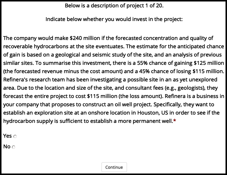
Figure A.25: An example of a project display in Experiment 4.
A.4.1.2.3 Follow-up
The follow-up questions were identical to those in Experiment 3 (see Section A.3.1.2.3), except that the portfolio number question identified the number of projects they saw as 20.
A.4.2 Results
A.4.2.1 Project Investment
The project investment data were analysed as in Experiment 2 (see Section 2.3.2). Figures A.26 and A.27 show the choice and proportion data, respectively. The difference between awareness conditions was not significant, both in the logistic regression \(b = -0.05\), 95% CI \([-0.22, 0.13]\), \(z = -0.53\), \(p = .595\), and in the t-test, \(d_s\) = -0.09, 95% CI [-0.33, 0.15], \(t\)(264) = -0.73, \(p\) = .464.
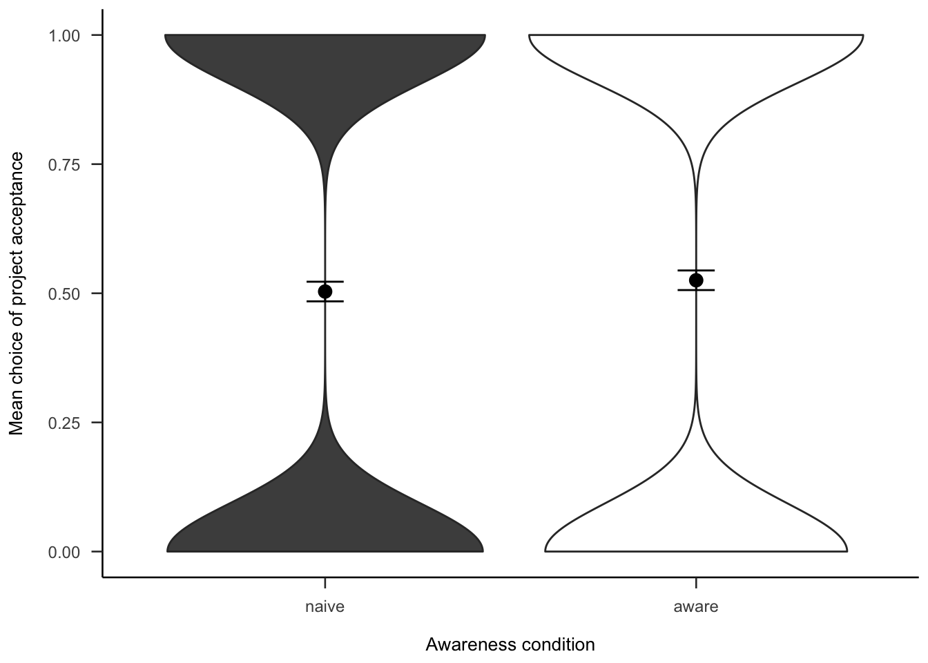
Figure A.26: Mean project acceptance for the awareness effect.
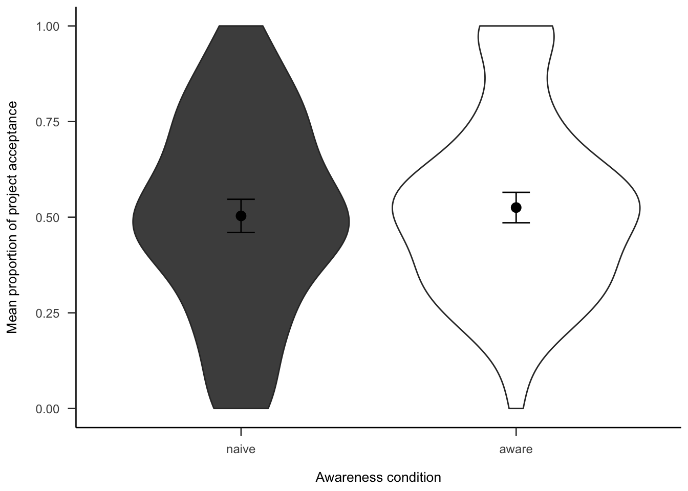
Figure A.27: Mean proportion of project acceptance for the awareness effect.
Further, Figure A.28 shows the choice data as a function of the order of the project in the sequence. As Table A.4 shows, there were no main effects or interactions.
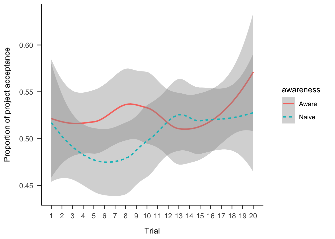
Figure A.28: Mean project acceptance by awareness and trial.
| Term | \(\hat{\beta}\) | 95% CI | \(z\) | \(p\) |
|---|---|---|---|---|
| Intercept | -0.01 | [-0.20, 0.17] | -0.12 | .907 |
| Awareness1 | -0.10 | [-0.28, 0.09] | -1.05 | .293 |
| Project order | 0.01 | [0.00, 0.02] | 1.66 | .096 |
| Awareness1 \(\times\) Project order | 0.00 | [-0.01, 0.01] | 0.29 | .775 |
A.4.2.2 Follow-up
A.4.2.2.1 Project Expectation
Participants were asked how many projects they expected to see. Figure A.29 shows that those in the aware condition reportedly expect to see more, \(d_s\) = -0.94, 95% CI [-1.19, -0.69], \(t\)(264) = -7.67, \(p\) < .001. However, this is likely to be due to the fact that they were told how many projects there were.
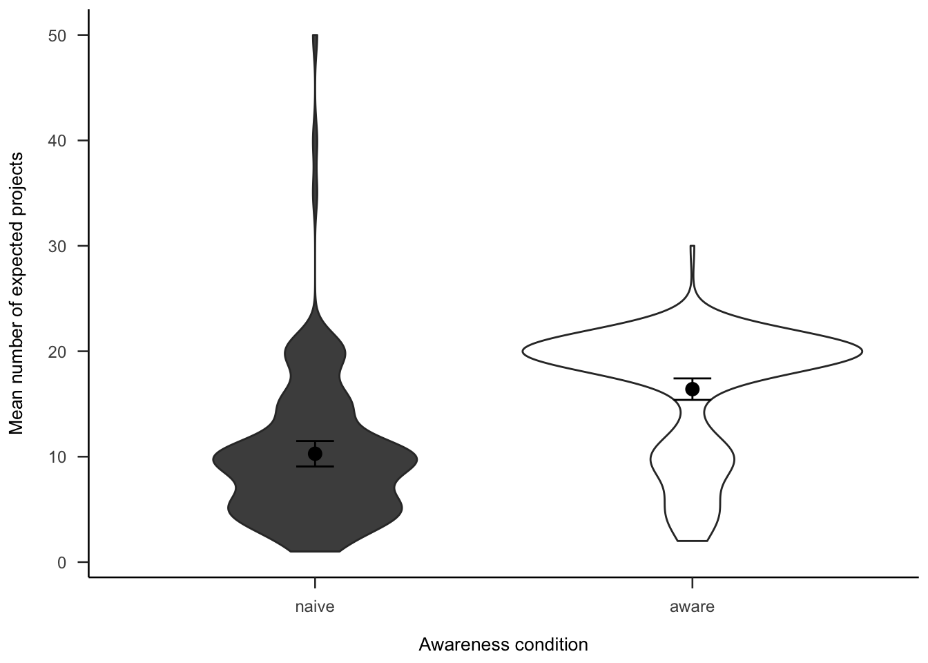
Figure A.29: Number of projects participants expected to see, by awareness.
A.4.2.2.2 Project Number
Participants were asked how many projects they thought they saw. Figure A.30 shows that overall people correctly estimated the number of projects, with higher accuracy for those in the aware condition.
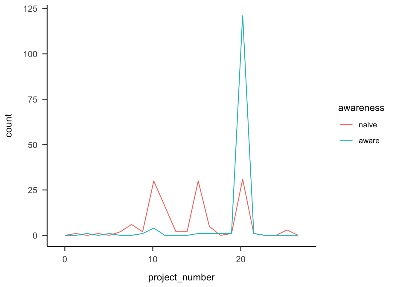
Figure A.30: Number of projects participants reported seeing, by awareness.
A.4.2.2.3 Portfolio Choice - Binary
Participants were then asked if they would rather invest in all or none of the projects. As Figure A.31, there was no significant difference between awareness conditions in wanting to invest in all of the projects, \(b = -0.09\), 95% CI \([-0.33, 0.15]\), \(z = -0.74\), \(p = .460\).
(ref:plot-aggregation-4-portfolio-binary) Mean choice of investing in all 20 projects for the awareness effect.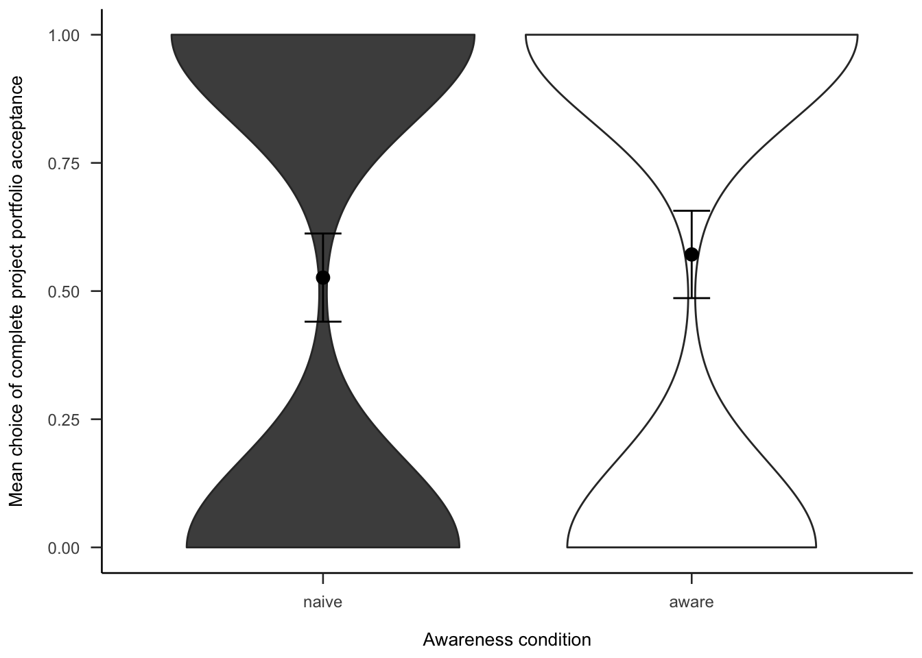
Figure A.31: (ref:plot-aggregation-4-portfolio-binary)
A.4.2.2.4 Portfolio Choice - Number
Subsequently, we asked participants how many projects they would invest in out of the 20 that they saw. As Figure A.32 shows, the difference between awareness conditions was not significant, \(d_s\) = -0.12, 95% CI [-0.36, 0.12], \(t\)(264) = -0.97, \(p\) = .334.
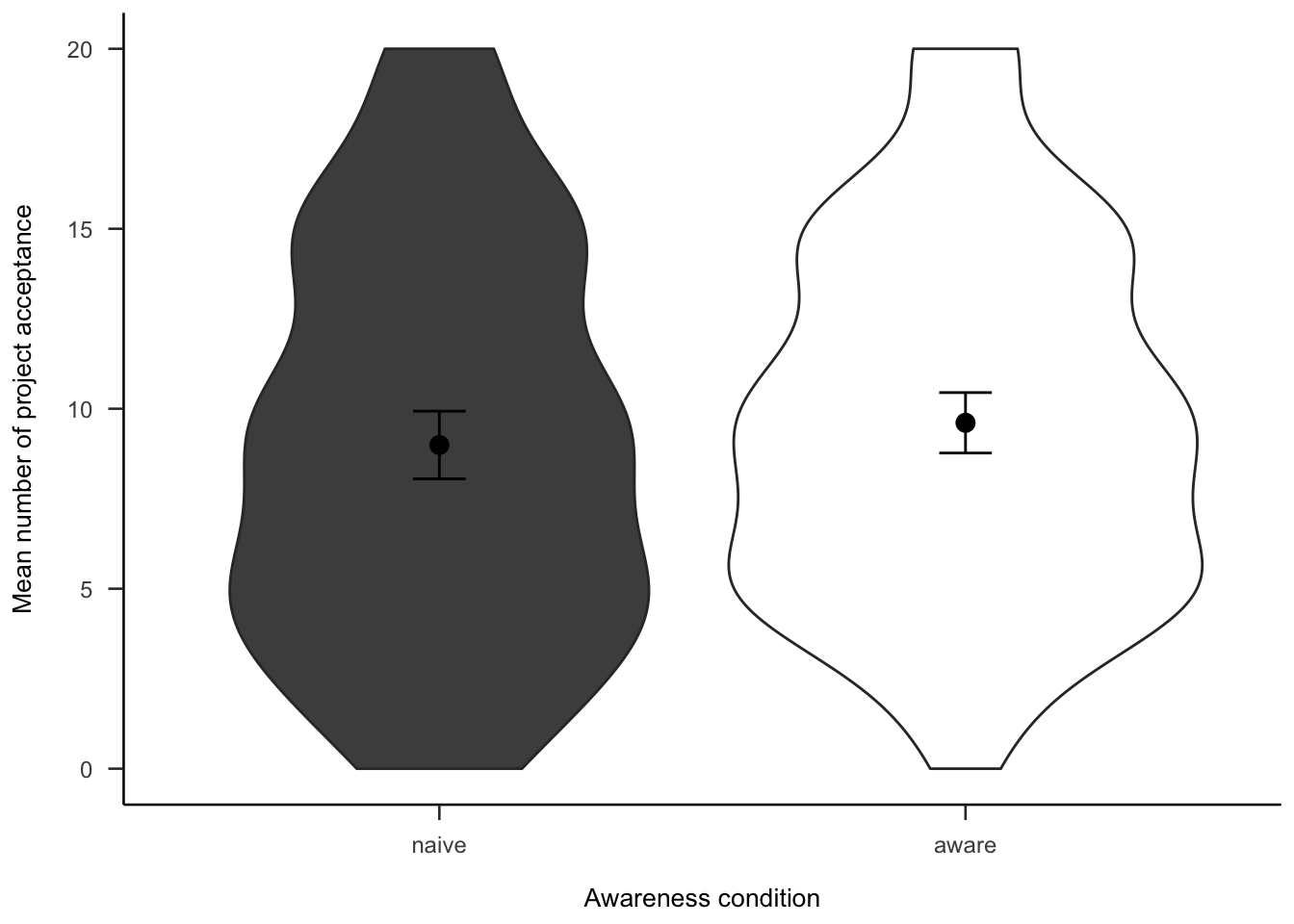
Figure A.32: Mean number of projects chosen in the follow-up for the awareness effect.
A.4.2.3 Gambles
Figures A.33 and A.34 show the overall people seemed to prefer gambles with higher probabilities of gain, sometimes regardless of expected value or value of the gain.
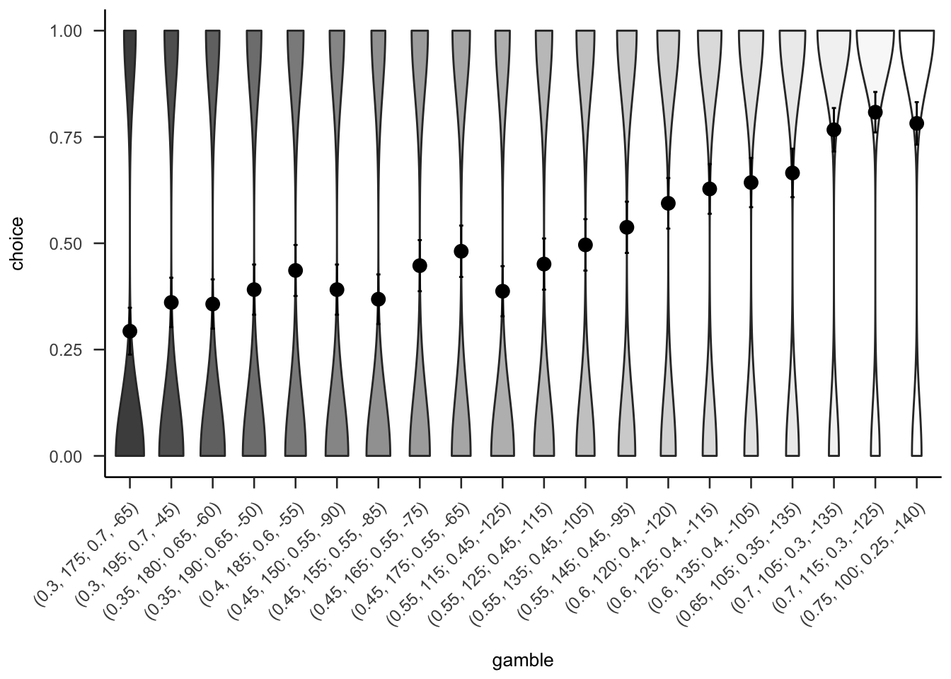
Figure A.33: Mean project acceptance for the 20 gambles. The format of the labels indicate: (gain probability, gain value; loss probability, loss value).
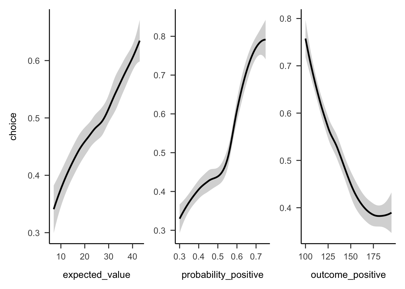
Figure A.34: Mean project acceptance for the gambles’ expected value, positive probability, and positive outcome.
A.4.3 Discussion
Experiment 4 did not find evidence for Hypothesis 2.4. There was no significant effect of awareness on project choice by trial. Participants in the aware condition were expected to become less risk averse as they continued with the experiment if they were using a strategy similar to the law of small numbers. The fact that this effect was not replicated in Experiment 4 might mean that the finding in Experiment 1 was due to the specific gambles used in that experiment, or statistical chance.
References
Champely, S. (2020b). Pwr: Basic functions for power analysis [Manual]. https://github.com/heliosdrm/pwr
Hong, Y. (2013). On computing the distribution function for the Poisson binomial distribution. Computational Statistics & Data Analysis, 59, 41–51. https://doi.org/10/gjscrd
Redelmeier, D. A., & Tversky, A. (1992). On the Framing of Multiple Prospects. Psychological Science, 3(3), 191–193. https://doi.org/10/ctw2k6
Samuelson, P. A. (1963). Risk and Uncertainty: A Fallacy of Large Numbers. Scientia, 57(98), 108–113. https://www.casact.org/sites/default/files/database/forum_94sforum_94sf049.pdf